This is Part 2 in the machine learning series, covering model training and learning from data. Part 1 covers an overview of machine learning and common algorithms.
How does an ML Algorithm actually learn?
There are many types of ML algorithms. In this post I will discuss supervised learning algorithms. These operate on labelled data, where each data point has one or more features (also known as attributes) and an associated known true label value.
The goal of supervised machine learning is to develop an algorithm that can learn from labelled data to train a model and then use the model to make accurate predictions on unseen test data. All without being explicitly programmed to do so.
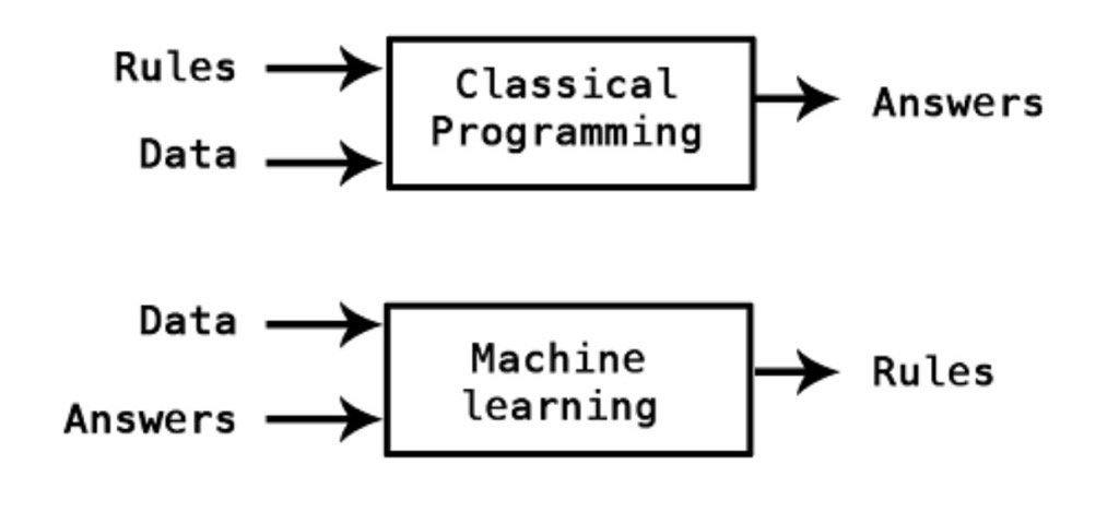 Classical programming contrasted with machine learning
Source: twitter.com/kpaxs
An algorithm learns from training data by iterating over labeled examples and optimising model parameters to minimise the difference between label predictions and true labels. It is this optimisation component that enables “learning”.
Some algorithms are quite simple with few parameters to tune (for example logistic regression) while others are very complex (for example transformer deep learning models). Below we’ll cover the trade-offs between different algorithms and the subtleties of training a model that generalises well for predictions.
Components of an ML Algorithm
A typical ML algorithm consists of a few essential components:
-
A loss function (which applies to a single training example)
-
An objective (or cost) function (usually the summation of the loss function over all the examples in the dataset)
-
An optimisation algorithm to update learned parameters and improve the objective function
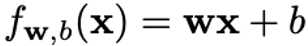
Let’s use a linear regression model as an example, where the weights (w) and bias (b) are the parameters of the model to learn, x is a single input data instance and f(x) is the prediction for x.
Here’s the linear model formulation:
 squared area loss function
And the components:
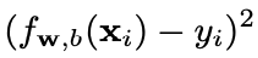
-
The squared area loss function (applies to a single training instance):
 linear regression model
The mean squared error (MSE) objective function applies to the whole dataset:
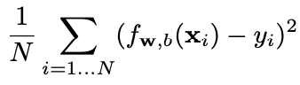 mean squared error (MSE) objective function
An optimisation algorithm. One possible example is Gradient Descent, since the objective function is differentiable. (Another option is a closed form solution, but that isn’t always solvable when the dataset is large).
Gradient Descent Optimisation Algorithm
Gradient Descent is a first-order iterative optimisation algorithm for finding a local minimum of a differentiable function. It’s commonly used to optimise linear regression, logistic regression and neural networks.
The basic idea behind gradient descent is to take steps in the direction of the negative gradient of the objective function with respect to the parameters. The negative gradient informs the direction in which the objective function is decreasing most rapidly, so taking a step in that direction should quickly reach a minimum.
There are several variations of gradient descent, such as stochastic gradient descent, which uses a random subset of the data to update the parameters in each iteration, and mini-batch gradient descent, which uses a small batch of data to update the parameters in each iteration.
It shouldn’t be confused with backpropagation, which is an efficient method of computing gradients in a directed graphs of computations (for example in neural networks).
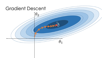 Gradient Descent
Source: www.samlau.me
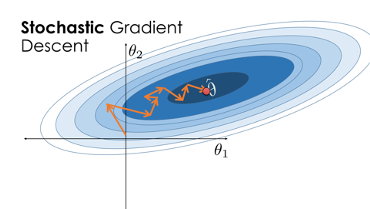 Stochastic Gradient Descent
Source: www.samlau.me
The No Free Lunch Theorem is a concept that states that there is no one model that works best for every problem. The theorem essentially says that if an algorithm performs well on a certain set of problems, then it must necessarily perform worse on others.
The assumptions of a great model for one problem may not hold for another problem, so it is common to try multiple models and find one that works best for a particular problem.
Under and Over-fitting
Underfitting and overfitting are common problems that can occur when training models.
Underfitting occurs when the model is too simple to capture the underlying patterns in the data. In other words, the model is not complex enough to fit the training data, and it performs poorly on both the training and testing data.
Overfitting occurs when the model is too complex and fits the training data too well, including the noise in the data. In this case, the model is not able to generalise to new, unseen data and performs poorly on the test data.
Both underfitting and overfitting can lead to poor performance and inaccurate predictions. The goal is to find the right balance between model complexity and performance on the training and testing data. Techniques such as cross-validation, regularisation, and early stopping can help to prevent overfitting and underfitting in machine learning models.
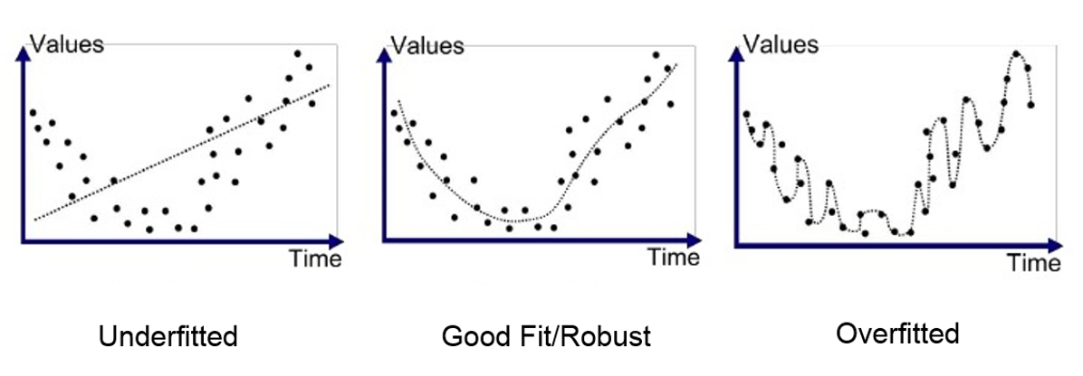 Examples of under/good/over fitting
Source: Anup Bhande
Bias and Variance
Bias and variance are two important concepts that relate to the ability of a model to accurately capture the underlying patterns in the data.
Bias refers to the error that is introduced by approximating a real-world problem with a simplified model. A model with high bias is unable to capture the complexity of the underlying patterns in the data and may result in underfitting.
Variance, on the other hand, refers to the error that is introduced by the model's sensitivity to small fluctuations in the training data. A model with high variance is too complex and may result in overfitting. In other words, a model with high variance is too sensitive to the noise in the training data and may fail to generalise to new, unseen data.
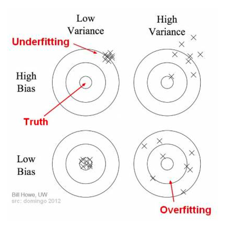 Bias/variance intuition
Source: Seema Singh
Bias / Variance Tradeoff
Bias and variance trade off against each other. This tradeoff is a central problem in supervised learning.
The goal is to find the right balance between bias and variance to achieve the best predictive performance on new, unseen data. Techniques such as regularisation, cross-validation, and ensembling can help to balance bias and variance in machine learning models.
Ideally, we want a model that accurately captures the regularities in its training data and generalises well to unseen data. Unfortunately, it is typically impossible to do both simultaneously.
-
Expected generalisation error is the sum of the bias and variance error
-
Overfitting: low bias, high variance
-
Underfitting: high bias, low variance
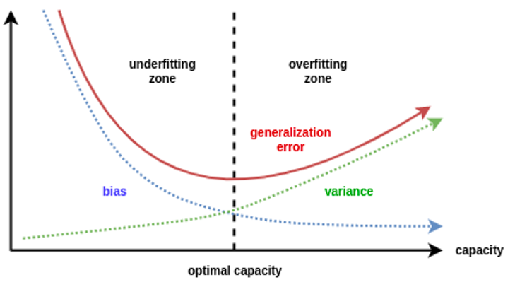 Bias/variance error decomposition
Source: Daniel Saunders
Training/Validation/Test Data Splits
Training, validation, and test data splits are used to evaluate the performance of a model on new, unseen data. These data splits are used to train the model, tune its hyperparameters, and evaluate its performance.
The training set is the part of the data that is used to train the model. It is the data on which the model is fitted, and its parameters are optimised to minimise the objective function.
The validation set is used to evaluate the performance of the model with different hyperparameter values and select the best set of hyperparameters.
The test set is the part of the data that is used to evaluate the final performance of the model. It is a new, unseen dataset that the model has not been trained on or used to tune hyperparameters. The test set is used to estimate the performance of the model on new, unseen data and to determine if the model is generalising well.
It is important to keep the test set separate from the training and validation sets to avoid overfitting and to obtain an unbiased estimate of the model's performance. If there is not enough labelled, cross-validation is another option.
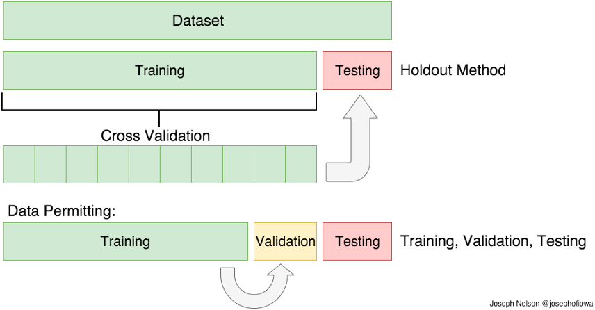 Data splits
Source: Adi Bronshtein
Hyperparameters
Hyperparameters in machine learning are model settings that cannot be learned during training but must be set before the training process begins. They control the behaviour of the model and can have a significant impact on its performance.
Hyperparameters are typically set by the user and are not learned from the data. They can include settings such as the learning rate, the number of hidden layers in a neural network, the number of trees in a random forest, the regularisation strength, or the kernel type in a support vector machine.
Finding the right hyperparameter values is essential to ensure that the model performs well on new, unseen data. They can be difficult to set, as their optimal values can depend on the dataset, the model architecture, and the specific problem being solved.
There are many approaches to hyper-parameter optimisation, for example:
-
Grid search – simple parameter sweep
-
Bayesian optimisation - builds a model of the function mapping from hyper-parameter values to the objective
Regularisation
Regularisation is an umbrella term of methods that force the learning algorithm to build a less complex model. It is any modification we make to a learning algorithm that is intended to reduce its generalisation error but not its training error.
Regularisation examples:
-
L1 regularisation (aka lasso regression) – adds the absolute value of the model coefficients as a penalty term to the loss function. (many coefficients tend to 0 which helps with feature selection)
-
L2 regularisation (aka ridge regression) – adds the squared value of the model coefficients as a penalty term to the loss function. (L2 is differentiable meaning gradient descent can be used to optimise the objective function)
-
For neural networks:
-
Dropout: randomly "dropping out" units during training
-
Batch normalisation: re-centering and re-scaling layer inputs
-
Learning Curves
A learning curve is a graph that shows how the performance of a model changes as the size of the training set increases or the model complexity increases.
Learning curves are used to diagnose the bias-variance tradeoff of a model and to determine whether the model is underfitting or overfitting. They can also be used to determine if more data will improve the model, evaluate the effect of regularisation, perform feature selection, and hyperparameter tuning on the performance of the model.
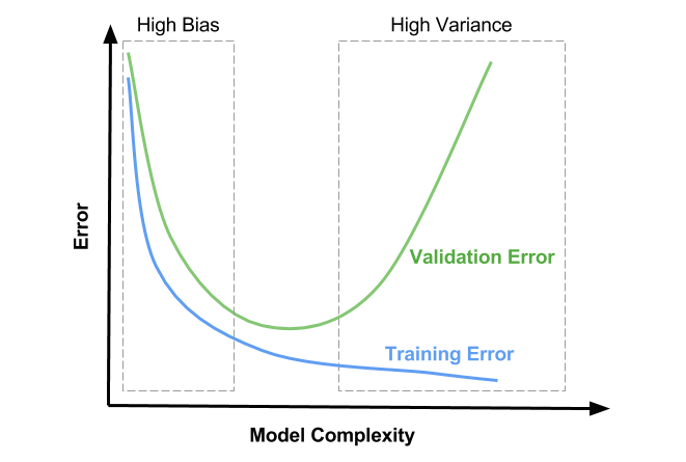 Model complexity learning curve
Source: Satya Mallick
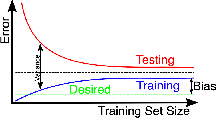 Training set size learning curve
Source: wikimedia
Assessing Model Performance
To assess the performance of a machine learning model, several evaluation metrics can be used. The choice of the metric depends on the specific problem and the type of model being used.
Here are some common evaluation methods and metrics:
-
Confusion matrix summarises predictions vs true labels
-
Precision: fraction of relevant instances among the retrieved instances
-
Recall: fraction of relevant instances that were retrieved
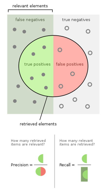 Precision and recall components
Source: wikipedia.org
-
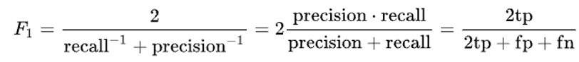
F1-score: balance between precision and recall
-
ROC curve: plot of model performance for all classification thresholds
-
AUC: Area under the ROC curve, provides an aggregate measure between 0 and 1 of performance across all possible classification thresholds
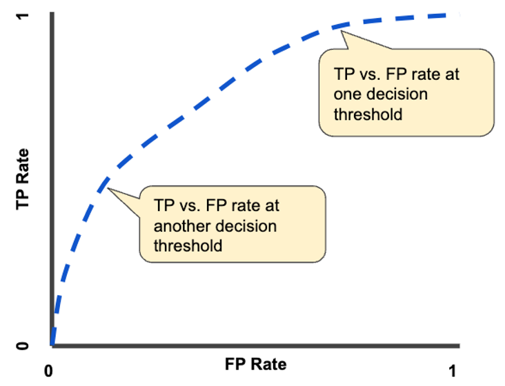 TP vs FP rate at different classification thresholds
Source: developers.google.com
Further Considerations
There are many further important considerations when training a good machine learning model. I plan to cover these in a future post. For now I’ll list
-
Handling imbalanced datasets with over & under sampling
-
Choosing a good objective function to optimise
-
Normalisation/standardisation of features
-
Prevent information leakage from training to test sets (especially with time series data)
-
Model interpretation & explainability
-
Data and model/concept drift over time
-
Model performance at training (and inference) time
Further Resources
Check out Part 3 of this machine learning series covering deploying machine learning models into a production system and maintaining them over time.
These are my recommended machine and deep learning lecture videos, all available via Youtube:
-
Stanford CS229: Machine Learning with Andrew Ng, 2018 (online notes)
-
Stanford CS230: Deep Learning with Andrew Ng, 2018 (online notes)
-
CS231n: DL for Computer Vision with Andrej Karpathy, 2016 (online notes)
-
MIT 6.S191 Intro to DL Home with Alexander Amini, 2022 (github repo)
-
UW-Madison STAT 451 Introduction to ML with Sebastian Raschka, 2021 (github repo)
Google also has a good foundational and advanced ML courses.
Additionally, here are some amazing machine learning notes by Christopher Olah that everyone should checkout: colah.github.io