What is Topic Modelling?
Topic modelling is a useful approach for automatically organising a large collection of documents into topics. Automatic is the key here - we don’t require predefined document labels nor even predefined topics to perform the organisation. Topic modelling falls under a broader collection of methods within Natural Language Processing and Machine Learning.
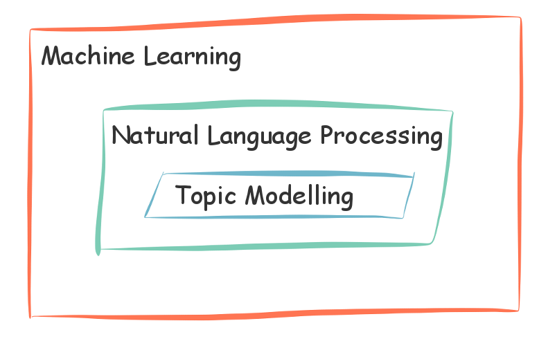 Topic modelling relation to NLP and ML
For example, thousands of New York Times articles (our collection of documents, also known as a corpus) can be organised into a number of topics. This could enable readers to visually explore stories within a particular topic or enable the publisher to recommend articles based on reader preferences.
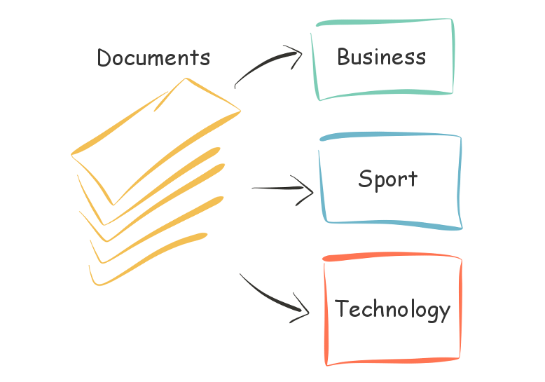 Topic modelling over a collection of documents
Many methods have been developed for topic modelling over the past few decades. Most methods rely on the fact that a document is typically about a particular subject and has words that frequently occur together. For example, an email planning your next holiday will likely contain the words ‘flight’ and ‘hotel’ more often than emails about other subjects. It is this statistical regularity that allows latent topics to be discovered, sometimes as if by magic.
The only data required for topic modelling is the text within each document. In machine learning terminology, this is an unsupervised learning method - meaning that we don’t require labelled data as is the case with supervised learning methods. The number of topics to automatically discover typically needs to be specified which can be tricky and may depend on how the results will be used. Interpretation of the discovered topics can also be tricky; while they can often be summarised by their most important words, they do not necessarily correspond to topics we expected to find.
The following sections will describe (in roughly chronological order of discovery) the intuitions behind a few different methods of applying topic modelling.
Topic Modelling Methods
Prerequisite: Preparing the documents
In order to discover topics within a corpus, the contents of all documents must be converted into a numerical format that becomes the input for a topic modelling method or algorithm. How this conversion is performed depends on a number of factors, for example, the chosen topic modelling method, the content of the documents themselves and also which language modelling simplifications are acceptable while still achieving the desired outcome.
One numerical format, that we will use below, is called a term-document matrix (where a term is simply a word from the vocabulary over all documents.) This format happens to discards word order and simply counts the number of occurrences of each term within a document. This simplification of ignoring word order (also known as a bag-of-words model) greatly reduces the complexity of representing the original documents and can still produce good results.
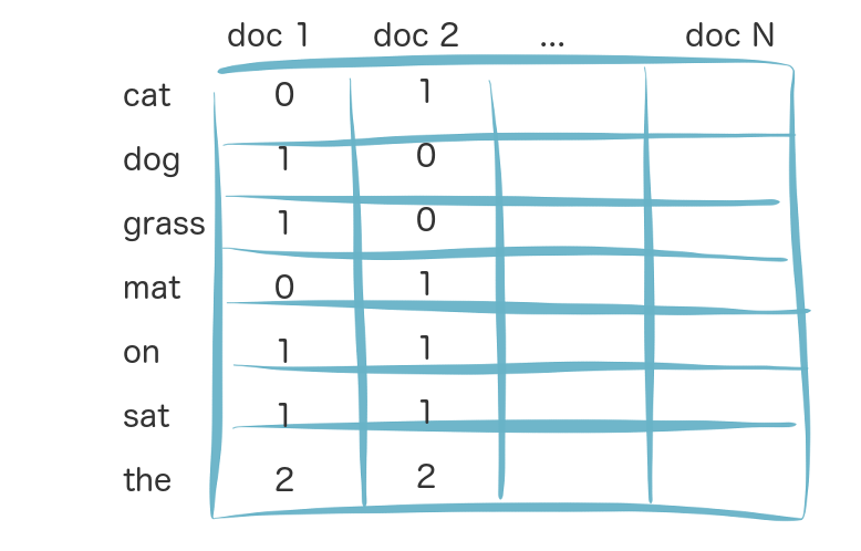 Simple term-document matrix example for 2 documents:
doc1: the dog sat on the grass
doc2: the cat sat on the mat
The term-document matrix is a sparse matrix containing mainly zeros (since documents typically don’t use all words) and represents each document as a column. Each entry is a count of the number of word occurrences in the document. While term-document matrices are common in information retrieval literature, for large datasets a document-term matrix having documents as rows can be easier to work with and is more common in software libraries.
The steps described here are very simple. There are many extensions that can be applied, for example, an entry in the term-document matrix can be extended to include the notion of term frequency–inverse document frequency (TF-IDF) which is a term weighting scheme. Regarding the vocabulary, in order to reduce the size of the term-document matrix, and also remove information that is often not useful, we can exclude common stop words (e.g. the, and, on) and likewise rare words that may only appear in a few documents. Additionally, word stemming can be applied such that only root words are included for analysis (e.g fished and fishes become fish.)
Method 1: Latent Semantic Analysis (LSA)
Latent Semantic Analysis is a method that was developed in the late 1980’s by Deerwester, Dumais and others 1. It takes as input a term-document matrix and factorises this into 3 new matrices which are able to jointly reconstruct the original matrix. This is achieved by applying a linear algebra method called Singular Value Decomposition (SVD) where the factorisation can be represented as M = UΣV’.
Each factored matrix gives us an insight in potential topics latent in the original term-document matrix. Specifically, matrix U maps words to a topic space, matrix V maps documents to the same topic space and matrix Σ is a diagonal matrix that tells us the ‘strength’ of each topic - whereby strong topics capture more variance in the underlying data.
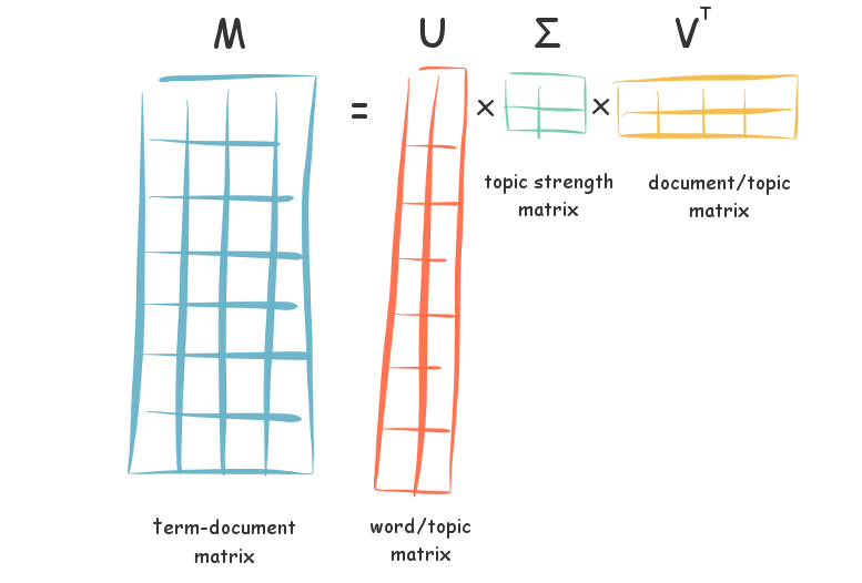 Singular Value Decomposition of a term-document matrix M
Knowing the strength (or variance) of the different topics is key. Strong topics allow us to model much of the original data while weak topics can be likened to modelling noise. Given this, we can choose to keep the top K topics and discard the rest. Specifically, a variant of SVD known as Truncated SVD does precisely this and is an instance of dimensionality reduction such that we find the most important aspects of the data to enable the best approximate reconstruction of the original term-document matrix. These important aspects are the topics we are seeking to model.
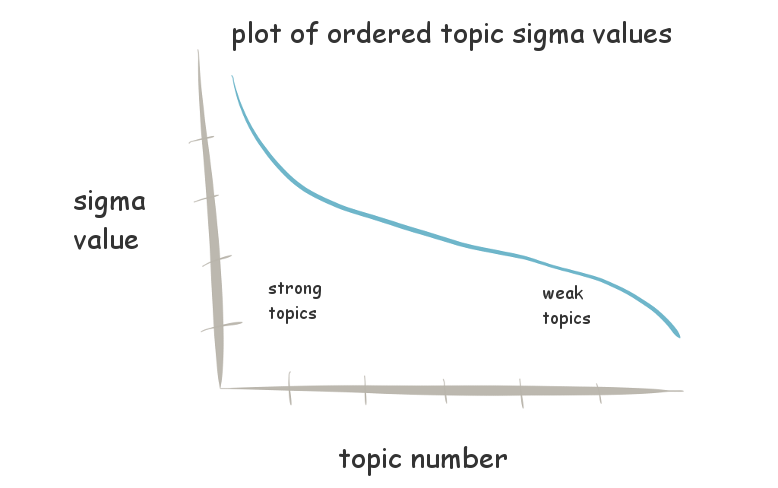 Plot of Topics (X axis) vs Topic Strength (Y axis) with topics ordered by strength
Choosing an appropriate number of topics to keep can be difficult and may be dependent on the problem domain you are modelling. There are several approaches, one of the simplest being to choose a cut-off value within the strength matrix Σ, either automatically or after plotting the values to identify where the values plateau.
Given we have our truncated matrix factorisation with K topics, we also have a vector representation of each document over the topics, namely the columns of ΣV’. Documents with similar topics tend to be close within this reduced latent space. The final step to topic modelling with LSA is to apply a clustering method (for example K-means or a hierarchical clustering algorithm) over these resulting vectors.
While LSA is simple to construct, a common criticism is that the model doesn’t explain why the matrix factorisation should generate good topics. The next method, PLSA, takes a different approach and attempts to solve this issue.
Method 2: Probabilistic Latent Semantic Analysis (PLSA)
Probabilistic Latent Semantic Analysis is a probabilistic version of LSA and was developed in 1999 by Hoffman 2. While PLSA and LSA attempt to solve a similar problem regarding topic modelling of a corpus, their approaches are very different. PLSA is a probabilistic generative model compared to LSA which is a deterministic model that uses linear algebra. Like LSA, PLSA works with a term-document matrix constructed from the collection of documents.
A probabilistic generative model describes a process of how data came to be via a sequence of probabilistic steps - in our case this is the story of how our documents may have been written or generated. Then, given this model or story, statistical inference is used to infer hidden/unobserved variables - which in this case happen to represent different topics.
The PLSA model assumes the following generative story, in which the actual parameter values will be inferred from the observed documents later:
- Randomly choose a document d with some probability: p(d)
- For each word in the chosen document d:
- Choose a topic t with some probability given the document d: p(t|d)
- Then choose a word w with some probability given the topic t: p(w|t)
The steps in this model and it’s variable dependencies can be shown using ‘plate’ notation in the following form:
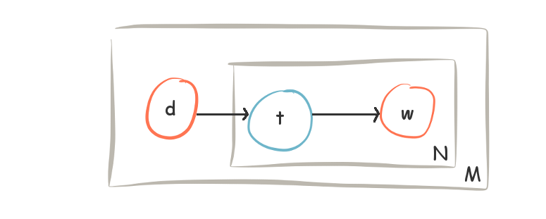 Plate graphic for the Probabilistic Latent Semantic Analysis model
In the PLSA model, we can see that choosing a word w is conditionally independent to documents given a topic (i.e. p(w|t) = p(w|d,t) which says that the probability of choosing a word given a topic is equal to the probability of choosing a word given a topic and a document.) The model also allows multiple topics within each document.
The next step is to determine the topic distribution over the documents by solving the model. Statistical inference is used to estimate the parameters of the PLSA model and give us a probability regarding all topics over each document (i.e. the probability of a topic given a document, p(t|d)). This essentially finds parameters that maximise the probability of generating the original observed term-document matrix. In practice, the Expectation Maximization algorithm can be used to estimate the parameters in an iterative manner.
There is a correspondence between the estimated probabilities of PLSA and the factored matrices of LSA, namely:
- Matrix M corresponds to the joint probability of a document and a word: p(d,w)
- Matrix U corresponds to the probability of a document given a topic: p(d|t)
- Matrix Σ corresponds to the probability of a topic: p(t)
- Matrix V corresponds to the probability of a word given a topic: p(w|t)
PLSA learns the probabilities of a topic, p(t), directly from the original data which can be a limitation if extending the model to new documents. In essence, PLSA is only a generative model for the corpus it is estimated on and not new documents.
Another potential issue is that the number of parameters grows linearly with the number of documents which can make solving the model computationally difficult for large corpuses and also lead to overfitting (however other estimation algorithms, for example Tempered EM, can help with this and improve generalisation as can extensions to the PLSA model itself.)
Even though PLSA can exhibit limitations regarding new documents and overfitting, in many experiments it outperforms LSA. The next method, LDA, extends the PLSA generative model to address these issues.
Method 3: Latent Dirichlet Allocation (LDA)
Latent Dirichlet Allocation was developed in 2003 by Blei, Ng, and Jordan 3. It is a generalisation of PLSA and overcomes some of its shortcomings. LDA is a probabilistic generative model similar to PLSA. However, unlike PLSA, LDA allows for additional information to be encoded with the use of probabilistic distributions over topics and words. Like the other methods presented, LDA operates with a term-document matrix.
The distribution that LDA uses to model topics and words is the Dirichlet distribution. This is able to model uncertainty when sampling from a fixed number of distinct categories and is a common prior in Bayesian statistics. LDA when applied to topic modelling typically uses a prior Dirichlet distribution for topics-per-document and another for words-per-topic.
The advantage of this approach is that the model is able to encapsulate the assumption that a document tends to cover only a small number of topics; this sparse topic property helps prevent overfitting of data, especially with a smaller corpus. A Dirichlet prior can also result in better word disambiguation and generally provides better assignment of topics over documents. If an uninformative flat (uniform) Dirichlet prior is used, the LDA model is equivalent to PLSA.
The LDA model assumes the following generative story:
- Choose number of words for the document from a Poisson distribution
- Choose topic proportions for the document from a Dirichlet distribution
- For each word in the document:
- Choose a topic t from a multinomial distribution with parameters θ
- Choose a word w from a multinomial distribution, conditional on topic t
The steps in this model and it’s variable dependencies can be shown using ‘plate’ notation in the following form:
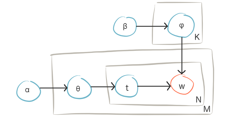 Plate graphic for the Latent Dirichlet Allocation model
Given that LDA allows for uncertainty through the use of prior distributions, it can be considered a Bayesian version of PLSA. Unfortunately this extra complexity comes at a cost. Estimation of LDA parameters is intractable and require computationally intensive algorithms to find approximate solutions, for example MCMC methods (such as Gibbs sampling, Metropolis-Hastings) and Variational Bayesian methods (an extension to the EM algorithm used to solve PLSA.)
Not all variables need to be inferred from the data. Some parameters can be set a priori and treated as hyperparameters, for example α and β parameters of the Dirichlet distributions can be fixed with values that depend on the number of topics and vocabulary size. Many extensions to LDA exist where additional variables are added to the model to capture different properties of documents.
While LDA will often produce better topic models than either LSA or PLSA, it still has shortcomings. The number of discovered topics is still fixed and the term-document matrix still does not capture sentence structure. Inference with LDA is also computationally expensive and tends not to scale well with an increasing number of documents. There are many ongoing areas of research regarding LDA including optimising inference algorithms, extending LDA to new domains, embedding LDA within other graphical models and integration with other NLP approaches like word2vec.
Wrap up
There are several other methods of topic modelling (e.g. Non-negative Matrix Factorization) and many extensions exist to the models detailed in this post. In a future post I plan to cover the empirical side of topic modelling including interpretation and evaluation of models, implementation via various code libraries (e.g. Scikit Learn and Gensim) and visualisation of resulting topics for a corpus (e.g using pyLDAvis). Additionally, I plan to produce a series of posts applying topic modelling to specific datasets and analysis of the results. Thanks for reading and I hope the information presented here is helpful for someone new to topic modelling.